-
Notifications
You must be signed in to change notification settings - Fork 8
Tutorial 2 Helicopter Blade Flapping Analysis
In this tutorial, will be animating a simple model of a single helicopter blade.
You can find the rigid model and a brief description of the model here
under "Helicopter blade analysis". However, we'll be using a slightly modified
version of the model that is available in the tests/bladeflap directory of the
Blendyn repository: the blade is this case is not rigid, but modeled
using a single 3-node beam element, just for the purpose of this tutorial.
The first thing that you want to do is, obviously, to simulate the model.
In the input file bladeflap.mbd provided in the repository, NetCDF
output is enabled by activating the related option in the control data
section of the input file
begin: control data;
	...
	output results: netcdf;
 end: control data;
This is not strictly necessary, but let's say highly recommended: it speeds up considerably the loading of the MBDyn output, and it enables plotting of MBDyn variables directly in Blender.
We're going to assume that the model has been simulated simply with
$ mbdyn bladeflap.mbd
so that the output files that we're going to import are called bladeflap.nc
and bladeflap.log.
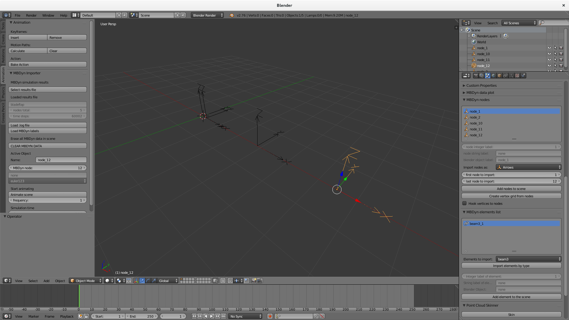
When the simulation has ended, fire up Blender and click on the Select results file button in the MBDyn Importer panel in the Animation Toolbar.
The context will be switched and you'll be asked to locate the output file of the
simulation: either a .nc file, in the case of NetCDF binary output, or a
.mov file, in the case we want to stick to the text output. The basename of
the output files, in our case bladeflap, will be shown under the Loaded results file label, if all went well.
The next step is click on the Load .log file button. The add-on will try to
load the bladeflap.log file, located in the same directory as the
bladeflap.nc file we previously selected. If it succeeds, the number of nodes
and the number of time steps will be shown under the results file basename.
It you have not modified anything else in the input file distributed with the
add-on, they will be, respectively, 5 and 60002.
We're now ready to import the nodes and the (recognised) elements in the scene.
Switch to the Scene Property panel and scroll down until you see the MBDyn nodes and elements lists
Click on the Add nodes to scene button to spawn 5 Empty Axes objects into the
scene, having initial position and orientation matching the one of the
corresponding MBDyn node.
You could already animate the Blender scene, for example setting the
frequency value to 100, and have a general idea of what was happening during
the simulation. Now we can import the beam element connecting node_10,
node_11 and node_12.
You can import the 3-no:qde beam element simply by clicking on the Add element to the scene button in the MBDyn elements section of the Scene Properties panel,
under the elements list. The 3-node beam element will be imported as a degree 2
(order 3) NURBS curve, with control points tied to the motion of the Empties
(please refer to this page to know why).
You can assign very easily a cross-section to the beam by defining a 2D curve as
a Bevel Object for the curve. Or, you can simply download an airfol profile
from Airfoil Tools, for example, and assign it automatically to the curve.
You can do so by downloading the Selig format dat file provided by Airfoil
Tools website (for example we're going to use the NACA23012.dat file available
here ) and clicking on the Load profile (Selig) button in the MBDyn beam props section of the Data Properties panel. Locate the profile file and
load it. It will be automatically assigned to all compatible Blender
Objects currently selected. In our case, to the beam3_1 object (please make
sure that the object is actually selected before loading the profile).
The Selig data format is extremely simple, as you can see from the excerpt below
NACA 23012  12%
 1.00003  0.00126
 0.99730  0.00170
 0.98914  0.00302
The first row contains the name of the profile, then all the other rows contain the coordinates of the points on the profile, the X-coordinate in the first column, the Y-coordinate in the second. Thus, this method is ceirtanly not limited to airfoil profiles, but can be used virtually any shape you want to import as the cross-section of beam (or rod) elements. Just be aware that all the points contained in the datafile will be considered as belonging to a single curve. You can, however, split a more complex profile into single connected curves, import them sepately, and then join them again in Blender before applying them as a bevel.
The final scene in this very simple tutorial looks like the following:
Happy simulations! :)


