TripleD

R-package to read and transform TripleD sample data to produce a database with presence-absence, density, and biomass data for benthic megafauna. The TripleD is a special quantitative sampling dredge produced and used by the NIOZ Royal Netherlands Institute for Sea Research.

This package contains all the code necessary to set up the TripleD database with time-series data collected by NIOZ. This package does not contain data; data can be requested from the NIOZ Data Archiving System (DAS).

The database output of the package can be visually interacted with using a developed Shiny app.

Installation

You can install the TripleD R-package including the HTML vignette by running the following command (beware you need to have the R-package devtools installed):

#install.packages("devtools")
devtools::install_github("dswdejonge/TripleD", build_vignettes = TRUE)

# Read vignette:
browseVignettes("TripleD") # click HTML

Contructing the database

Set up your working directory as follows in order to start with the NIOZ TripleD database:

1. Go to the NIOZ Data Archiving System (DAS) and request the formatted TripleD data CSV files.
2. In your working directory create a folder called 'inputfiles'. Within this folder you have to create two other folders called 'Species' and 'Stations'.
3. Put the CSVs with all species data in the folder 'inputfiles/Species' and the CSVs with all station data in the folder 'inputfiles/Stations' (do not put any files in these folders that are not csv data files formatted for the TripleD database).
4. Add and run the following R-script to your working directory:

# Load the library
library(TripleD)

# Loads all CSVs, checks format, and stores an R dataframe 
# in the newly created folder 'data'.
# Should not throw errors if the CSVs taken directly from DAS are used.
construct_database(in_folder = "inputfiles")

# Load the bioconversion CSV and check the input format.
check_bioconversion_input()

# Collect bathymetry from NOAA and taxonomy from WoRMS
collect_from_NOAA()
collect_from_WORMS()

# Prepare the bioconversion file to use (add valid taxon
# names and calculate mean conversions for each higher taxon)
prepare_bioconversion()

# Add extra data to the intial database (taxonomy, water depths
# from bathymetry, track lengths from coordinates and ticks,
# bearings, and ash-free dry weight using conversion data)
complete_database()

# Finalize database, by aggregating data, selecting relevant columns, and
# calculating final densities and biomass per sampling station.
finalize_database()

# There is a database with density and biomass data 
# per taxon per station.
load("database.rda")

# View definition of each database column.
att_database

# Extract a community matrix for ecological analysis,
# e.g. Ash-Free Dry Weight per m2 for all species.
CM <- get_community_matrix(database, "species", "Biomass_g_per_m2")

# There is also a database with individual size measurements 
# and weights per taxon.
load("database_individuals.rda")

# View definition of each database_individuals column.
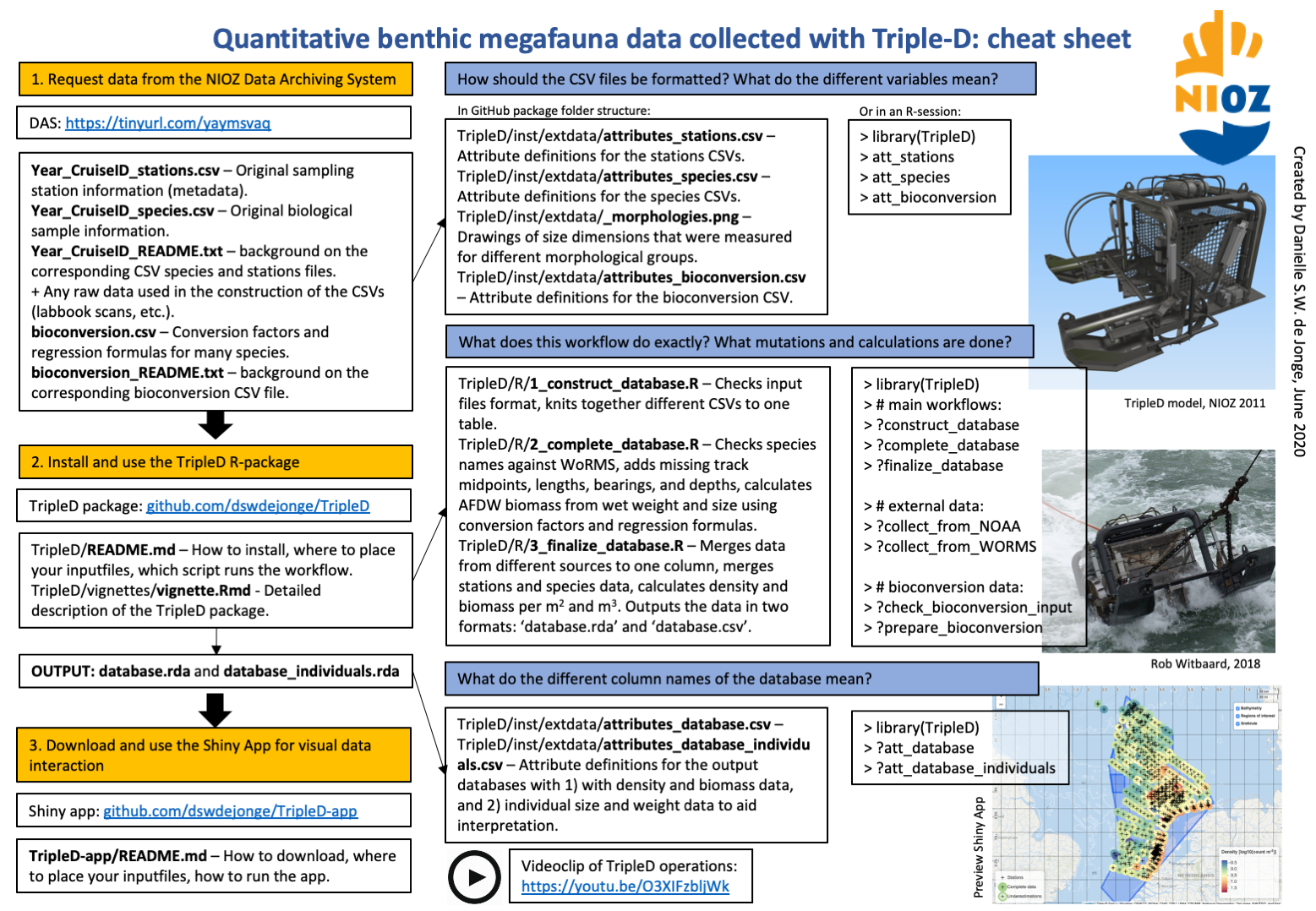
att_database_individuals

Cheat sheet

If you feel lost with the workflow and all the files, use this cheat sheet:

Size dimension

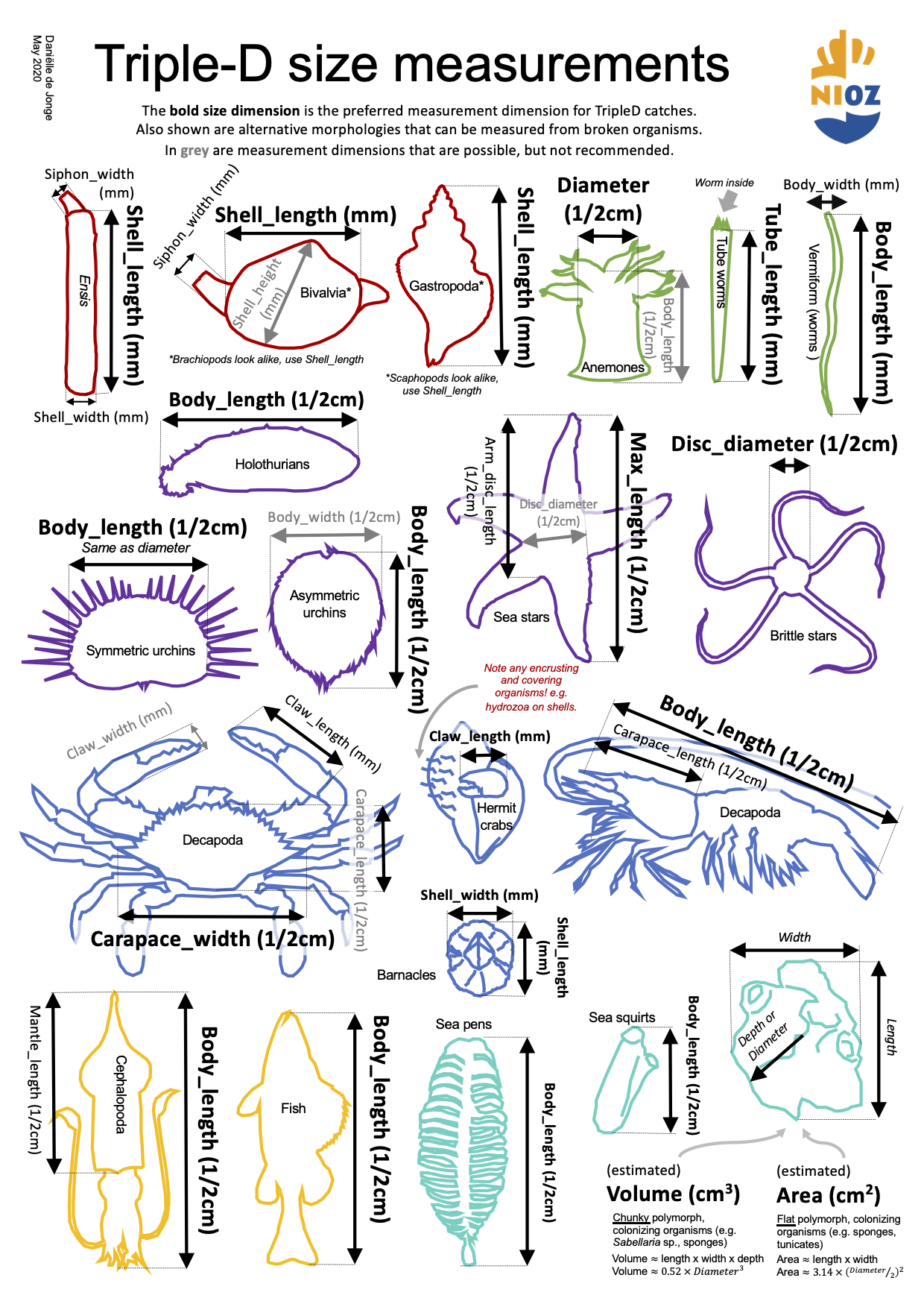
A quick reference and reminder of which size dimensions are measured for different morphological groups. The names in the diagram correspond exactly with the names in the species CSVs and bioconversion CSV that can be requested from the NIOZ Data Archiving System.