This tool is designed to help preprocess pupil signal from any eye-tracker (ET). This tool includes an automatic blink removal algorithm and a manual plot editor.

The main feature of this program is to linearly interpolate over artifacts, as determined by detecting significant changes in the pupil velocity (top plot). The endpoints of these changes in velocity are marked with a pink dot (onset) and red dot (offset). These endpoints are mapped onto the raw pupil (gray plot in the bottom panel, only the blink events are not obscured). The program linearly interpolates across these endpoints and generates the "cleaned" pupil timeseries (green plot).
Other features of this program are described below (WIP).
Table of Contents
- Installation (2 options)
- Pupil Preprocessing Overview
- Removing Blinks and Artifacts (Automated)
- How Does The Blink Removal Algorithm Work?
- Disclaimer
- Crediting
- Author
Use the standalone desktop program if you don't want to worry about dependencies and don't mind the large download size. Visit the latest release page and download the installer file that matches your operating system. Launch the installer on your local drive and follow the instructions to complete installation.
Running from the source code may be easier, provided that you already have these dependencies:
- Matlab (tested on 2019a and later)
- Signal Processing Toolbox
- Statistics and Machine Learning Toolbox
You can download the source code if you want to use the algorithm in your own script or if you want to run the app directly through Matlab. Simply clone or download this repository, making sure that the .m and .mlapp files are located in the same directory.
The project is written and tested on Matlab 2019a. The .mlapp file might not work with older Matlab versions due to use of uicomponents that were introduced in later Matlab versions. If you have an older version of Matlab and/or don't want to deal with dependencies, it may be easier to install the standalone program.

ET-Remove-Artifacts can be used on pupil timeseries data from any eye-tracker. But first, the raw data needs to be formatted as a Matlab data structure in a specific way (described in the next section). Once properly formatted, the pupil data can be loaded into the ET-Remove-Artifacts application. The app will automatically detect and linearly interpolate over blinks and other artifacts in your pupil timeseries. You can easily view the results of the blink removal algorithm in the app. If needed, you can also use the manual plot editor to interpolate over missed artifacts or impute longer sections of noisy data with missing data indicators (NaNs).
Your raw pupil data needs to be formatted as a Matlab data structure with the variable name S. The variable S then needs to be saved as a .mat file.
At a minimum, the data structure S needs to include the following required fields:
S
└── data
    ├── sample
    └── smp_timestamp
S.data(required): contains the raw pupil dataS.data.sample(required): the raw pupil values stored as a Nx1 numerical arrayS.data.smp_timestamp(required): the sample timestamps (in seconds) stored as a Nx1 numerical array (timestamps must be converted to seconds!)
Additionally, the data structure S may also include these optional fields:
S
├── data (required)
│   ├── sample (required)
│   ├── smp_timestamp (required)
│   ├── valid (optional)
│   ├── message (optional)
│   └── msg_timestamp (optional)
└── filter_config (optional)
S.data.valid(optional): the valid/invalid sample tag provided by some eye-trackers stored as a Nx1 logical array (1 = valid, 0 = invalid)S.data.message(optional): any task event label relevant to the sessionS.data.msg_timestamp(optional): the timestamps corresponding to the event labels inS.data.messageS.filter_config(optional): optional field that stores the configuration settings for the blink removal algorithm
After creating your data structure, save it as a .mat file (e.g., save('name_of_file.mat','S')).
- The
smp_timestampvalues need to be in seconds. If your raw data timestamps are in a different unit (e.g., Eyelink uses ms), they need to be converted to seconds. - The arrays in the
sample,smp_timestamp, andvalidsub-fields need to be the same size (Nx1 where N is the number of samples). - The
validsub-field should be an array of 1's and 0's, where 1's indicate the sample is valid. Some eye-trackers record invalid samples as 1's, so make sure to invert these in that case.
(TODO: add scripts for other eye-tracking formats)
The provided example scripts can be used as templates for formatting your eye-tracking data.
ReadRawData_Script.m is an example script showing how to read in raw data (using the included ET_ReadFile.m function) and format the data structure S to be compatible with ET-Remove-Artifacts. To view an example of a properly formatted data structure, load the provided Example_Data_Input.mat file (example data from an SMI eye-tracker). This file was created from the raw data files and code provided in the RawData2Structure folder.
If running the standalone desktop app, simply launch the app like a normal desktop program.
If using the source code, simply run the ET_RemoveArtifacts_App.mlapp (e.g., drag and drop the file into your Matlab command window).
Once the app opens, you can load your .mat file from File -> Load data structure. Then select and open your .mat file (see below).

Upon loading your data, the app detects if the file was previously processed by ET-Remove-Artifacts. If so, the program will not modify the data and will simply display your existing preprocessed pupil results. Otherwise, the program automatically applies the artifact removal algorithm using the default settings.
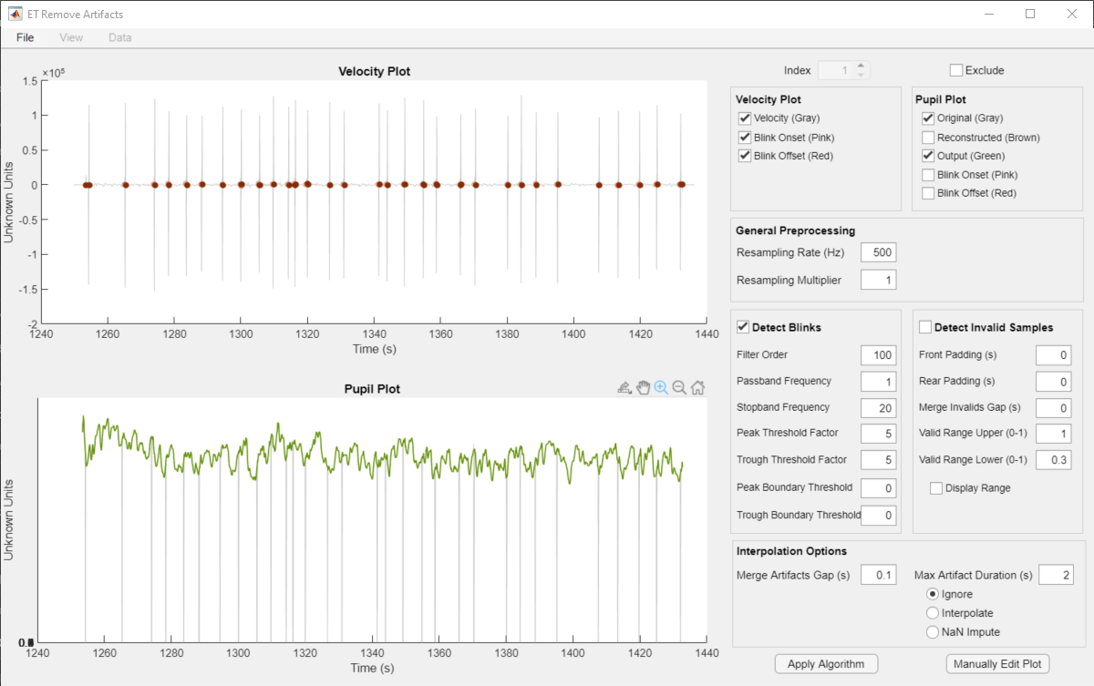
By default, the Pupil Plot displays the preprocessed Output timeseries (Green) overlaid on the Original timeseries (Gray). The Blink Onset (Pink) and Blink Offset (Red) are the start and end points of artifacts detected by the algorithm. The Velocity Plot displays the velocity or temporal first derivative of the original pupil timeseries. Blink Onset and Blink Offset are also plotted on the Velocity Plot. To interact with the plots, hover over the axes to reveal plot tools, which you can use to zoom and pan.
(show an example plot)
Click the up or down arrow next to the Index field to navigate through the other pupil datasets stored in your data structure. The index refers to the index of the data structure S that is currently being displayed.
Although the default settings for the blink removal algorithm should work for most pupil recordings, ET-Remove-Artifacts comes with some algorithm options that you can adjust to fine tune your results. We will describe all the algorithm options in the following sections, but you will likely only need to adjust a few of the settings.
These should be adjusted before you adjust the options in the other panels. Unless your eye-tracker's sampling rate is very high and you're encountering slow performance, you can typically leave Resampling Multiplier set at 1.
- Resampling Rate: the sampling rate (in Hz) of your preprocessed data. Typically, you would set this as the sampling rate of the recording from your eye-tracker. However, you can also use this to down/up-sample your data if you desire (if you're file size is too large to handle, you may want to downsample).
- Resampling Multiplier: the multiplier (value between 0 and 1) affects the temporary sampling rate of the data passed into the algorithm. The program resamples the data to the Resampling Rate*Multiplier and runs the algorithm on the temporarily resampled data. The data will then be resampled back to the original Resampling Rate. For eye-trackers with a very high sampling rate (e.g., > 500 Hz), downsampling your data for the algorithm would help speed up computing time. For example, if your Resampling Rate is set at 1000 Hz, you can set your Resampling Multiplier is 0.2 to get a temporary sampling rate of 200 Hz when running the algorithm.
Select the checkbox next to this panel to detect blinks in the pupil signal.
- Filter Order (must be an even integer): By default, the Filter Order is set at 20% of the Resampling Rate. Larger Filter Order values create a "smoother" velocity plot, but may suppress the blink velocity patterns if it is too large.
- Passband Frequency (Hz): Lower frequency constraint of the bandpass filter.
- Stopband Frequency (Hz): Upper frequency constraint of the bandpass filter.
- Peak Threshold Factor: Thresholding of a peak's amplitude in standard deviations above the mean velocity. Peaks whose amplitudes exceed this threshold are classified as an artifact peak.
- Trough Threshold Factor: Thresholding of a troughs's amplitude in standard deviations below the mean velocity. Troughs whose amplitudes exceed this threshold are classified as an artifact trough. A "blink" is characterized as an artifact trough followed soon after by an artifact peak.
- Velocity Threshold (+): Thresholding to find the point along the artifact peaks used to identify blink offsets. Smaller positive thresholds delays the blink offset, increasing the tail end of the interpolated region (and vice versa).
- Velocity Threshold (-): Thresholding to find the point along the artifact troughs used to identify blink onsets. Smaller positive thresholds makes the blink onset occur earlier, increasing the front end of the interpolated region (and vice versa).
The velocity plot (i.e., 1st derivative of the raw pupil data) is created by applying a differentiator filter. The first 3 options (Filter Order, Passband Frequency, and Stopband Frequency) control the design of the filter used when taking the 1st derivative of the raw pupil signal.
The algorithm then detects peaks and troughs in the velocity plot. Peaks and troughs whose amplitude exceed the Peak Threshold Factor and Trough Threshold Factor, respectively, are identified as artifacts.
Finally, the Velocity Threshold (+) and Velocity Threshold (-) options fine-tune the placement of the endpoints around each of the identified artifactual peak-trough periods.
(TODO - Figure of a blink profile to describe the thresholds)
Some eye-trackers also tag whether or not each recorded sample is valid, or provides a confidence metric for the sample quality. This information can be used in conjunction with the blink detection algorithm.
- Front Padding (s): Padding prior to the onset of invalid periods
- Rear Padding (s): Padding after the offset of invalid periods
- Merge Invalids Gap (s): If two invalid periods fall within this value, the entire period between the two invalid periods are merged into one invalid period
- Valid Range Upper (0-1): Samples above this value (fraction of the range of pupil values in this recording) are tagged as "invalid samples"
- Valid Range Lower (0-1): Samples below this value (fraction of the range of pupil values in this recording) are tagged as "invalid samples" (e.g., if this is set at .3, any sample with a value below .3 of the pupil range is an "invalid sample")
The Front Padding and Rear Padding options control the amount of padding around invalid periods that the program will interpolate over.
The artifacts identified by the blink detection and invalid detection portions of the algorithm are merged so that any overlap is treated as the same artifact.
- Merge Artifacts Gap (s): If two artifacts (could be a blink or invalid period) fall within this value, the entire period between the two artifacts are merged into one artifacts
- Max Artifact Duration (s): If an artifact exceeds this value, the program will either Ignore, Interpolate, or NaN Impute across this artifact (depending on the option that you select). Ignoring simply leaves the artifact alone and the raw pupil data is preserved. Interpolate linearly interpolates over the artifact. NaN impute replaces this artifact with NaNs.
Let's take a look at how the program handles pupil data recorded at 500Hz from an EyeLink eye-tracker (eyelink_example.mat). With the default options, the algorithm does a decent job of cleaning up most of the blink artifacts.

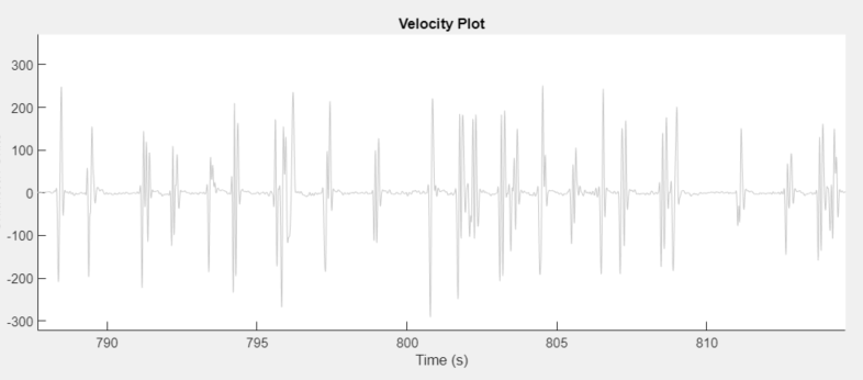
However, a few blink events were missed (e.g., at 1300s). Zooming into the the velocity plot around 1300s, we see that the reason for this miss is that there are two separate onset/offset pairs (so the blink is being treated as two successive blink events).

This can be handled several ways. The easiest in this case is to just add a small duration to the Merge Artifacts Gap (s) field. For example, setting it at 0.1s tells the algorithm to merge any two artifacts that are separated by less than 0.1s.
This results in an output (Green Line) that interpolates over every single blink artifact in the recording.
Recordings from some eye-tracking systems may yield atypical blink patterns. Let's take a look Example_Data_Input.m, which contains recordings from a 120Hz SMI eye-tracker, to see how the algorithm handles atypical blinks.
For example, zooming into a section of the raw pupil data, it's clearly difficult to provide a single set of properties that describes the all the blink events. Each blink event has a series of noisy, rapid fluctuations and even includes some spikes.

It's also difficult to qualitatively describe what the blink profiles look like in the corresponding velocity plot.
Applying the default options, we can see that the algorithm still does a decent job identifying the onset and offset (Pink and Red Dots, respectively) of each blink event. It is still able to yield an output (Green Line) that interpolates across the atypical blink events, with all their noise and spikes.

As seen in this example, the algorithm is not constrained to identifying typical blinks, and is fairly robust at handling all sorts of artifact patterns.

The manual plot editor is designed to complement the blink removal algorithm. At this stage of preprocessing, best practice is to dissociate the eye-tracking data from subject info and behavioral data.
Even though the blink removal algorithm adequately removes most of the blink events, there may be unusual artifacts that remain undetected by the algorithm. Some pupil data may have periods of "messy signal" (e.g., head movement + eye closing), and the algorithm may do a poor job at interpolating across these artifacts. The plot editor allows you to remove undetected artifacts or redo interpolation.
Once you are satisfied with the output of the blink removal algorithm, press the Manually Edit Plot button to launch the Plot Editor. The Axes Control panel allows you to pan through your plot as well as change the scale of the plot viewer. The Plot Editor Tools panel consists of the tools you'll need to edit your plot.
To edit your plot, you'll select the Start Point and End Point of the region you want to reconstruct. There are 3 functions you can apply to this region:
- Interpolate - linearly interpolates over the select region.
- Re-populate - replaces the selected region with original (non-reconstructed) data.
- NaN Data - replaces the selected region with NaNs.
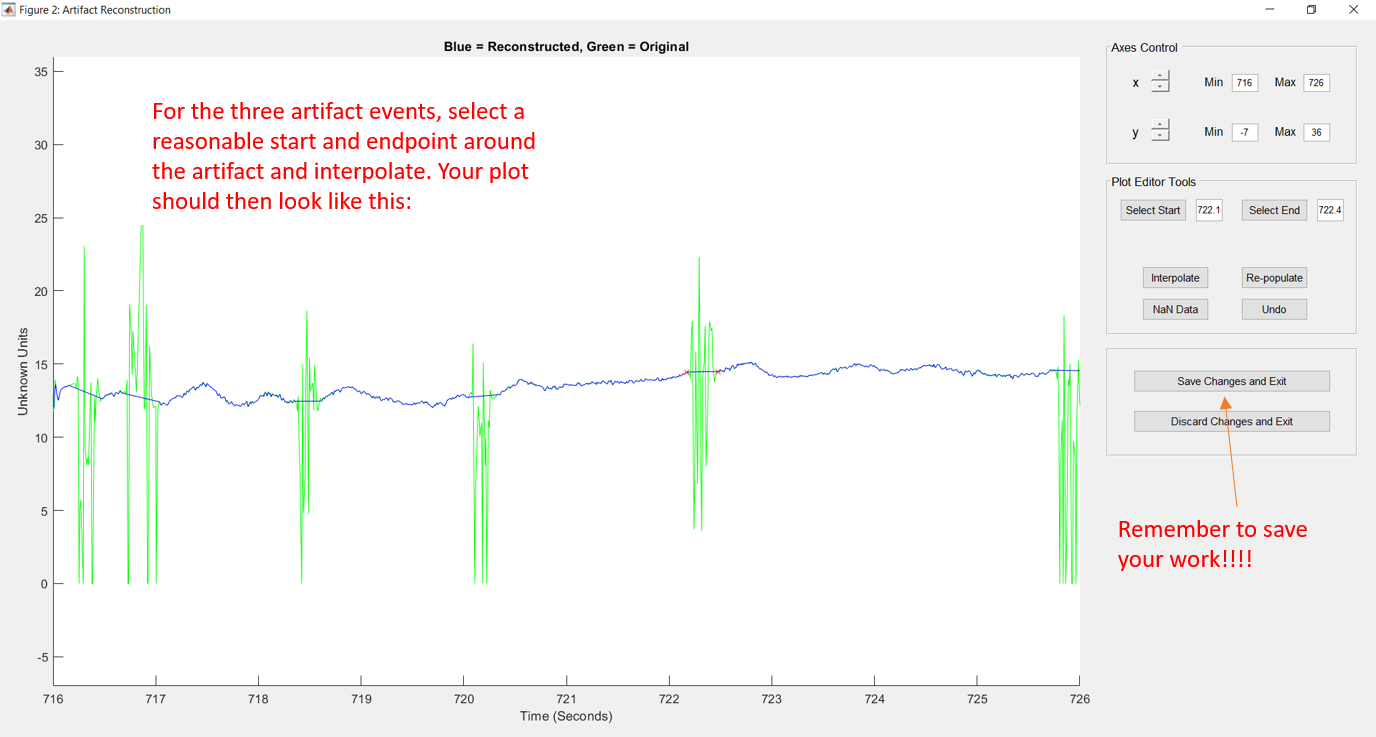
Here's an example of how you would use these tools:


Here's a different example:

To make this editing process more convenient, the plot editing tools are bound to keyboard hotkeys:
- WASD: arrow keys to navigate plot (AD: pans horizontally; SW: pans vertically)
- Q: select start point
- E: select end point
- Z: Interpolate
- X: Re-populate
- C: NaN Data
Some of the common cases that you would come across when editing your plots:
- An artifact in your signal that is untreated by the algorithm - select endpoints around the artifact and interpolate.
- An artifact in your signal is treated by the algorithm, but poorly done - select endpoints around the algorithm's interpolated region and re-populate the data. Then reselect the endpoints to better capture the artifact and interpolate over the reselected endpoints.
- An artifact or series of artifacts that is greater than 2-seconds in duration - select endpoints that cover this region of "messy" signal and replace with NaNs.
Load Example_Data_Final.mat to see what the final cleaned pupil data looks like after going through the entire algorithm + edit process.
Here, I replace that messy regions that are longer than 2-seconds with NaNs rather than interpolate. Later on in my analysis, I'll set criteria for trial exclusions based on the NaNs in the data. An example of this criteria may be: if the missing data occurs during a critical period of interest, exclude the trial. Or, if more than 50% of the pupil data in the trial is NaNs, exclude the trial.
Ultimately, defining the cut-off between interpolating and replacing with NaNs depends on your study design. Are your stimuli events long or short? What is the typical duration of the pupillary response you're interested in? The shorter the duration, the more stringent you're criteria for replacing data with NaNs. Typically, if I am unsure of whether to replace with NaNs or interpolate, I err on the side of replacing with NaNs.
When using this GUI, I suggest saving your output data structure under a different filename and making changes to that file. To do so: after loading in your input data structure, select the Save As button and save a copy of your data structure under a different file name. From then, whenever you restart the GUI, make sure to load in the new file and not the original input file.
The blink removal algorithm is based on the process described by Sebastiaan Mathot: www.researchgate.net/publication/236268543_A_simple_way_to_reconstruct_pupil_size_during_eye_blinks
For typical behavioral studies, the acquired pupillometry data is a slowly varying signal with occasional phasic changes in response to behavioral events. This slowly varying signal is interrupted by intermittent blink artifacts, which are characterized as a sudden decrease in pupil size followed by a sudden increase. Thus, we're able to detect blink events by looking at the velocity plot of the pupil signal. During periods of slowly changing signal, the velocity fluctuates around 0. In contrast, blink onsets are characterized by large negative velocities and blink offsets are characterized by large positive velocities.
Steps:
- Resample data
- Generate velocity profile by taking a filtered derivative of the raw pupil data
- Detect blink onsets/offsets by identifying peaks and troughs in the velocity profile
- Interpolate over blink onset/offset end points
For an additional reference, please see this excellent write-up documenting the entire preprocessing procedure from Isaac Menchaca: https://isaacmenchaca.github.io/2020/04/12/PupillometryPreprocessing.html
The tools in this repository and the preprocessing steps described above are designed with my own projects in mind. The guidelines expressed above should be taken as suggestions based on my own experiences and are not standardized rules for pupillometry preprocessing.
If using the toolbox as part of your pupil preprocessing pipeline, please consider citing the following reference:
Mather, M., Huang, R., Clewett, D., Nielsen, S. E., Velasco, R., Tu, K., Han, S., & Kennedy, B. L. (2020). Isometric exercise facilitates attention to salient events in women via the noradrenergic system. Neuroimage, 210, 116560.
- Ringo Huang - ringohhuang at g dot ucla dot edu
Feel free to reach out to me with questions regarding this tool or pupil preprocessing. Good luck!
👽📞🏡